Data Science: Everything You Need to Know About Using R for the Very First Time

Data Science: Everything You Need to Know About Using R for the Very First Time

Emily Halford 04/10/2020 11
Using R for the Very First time? Here is Everything You Need to Know

I was recently tasked with familiarizing an intern with R. As I thought about how best to direct him, I remembered how much I struggled to get my footing when R was entirely new to me.

I initially found so many great resources that explained various packages, best practices, and analyses, but I didn’t even know where to type my code! I eventually pieced together a general understanding of R usage via YouTube videos and felt like I was moving along successfully.

Then I was fortunate enough to take a fantastic R-based Data Science source in grad school and realized that my code was a mess. I didn’t know that R Projects and R Markdown files existed, so all of my code existed in poorly-organized scripts on my desktop. I backed up my work by emailing copies to myself and utilized variable names and spacing that make me cringe now. That course helped me learn how to create code that not only runs, but that is reproducible and which facilitates effective collaboration on my data analytics team.

Hoping to help this intern avoid my initial mistakes, I compiled the following guide for getting started with R. It is designed for complete beginners — the first section actually covers where to install the software! I made sure to include many of the important lessons that I learned in that Data Science course, and therefore frequently referenced the course website in the creation of this guide. I share this link not only to give credit to Jeff Goldsmith for his ideas, but also to provide a very useful resource for those looking for instruction that extends beyond the material covered here. This guide is certainly not exhaustive, but should get you up and running in R with a good workflow!


1. Installing Software

First, you’ll want to install both R and RStudio!

R download link: https://cloud.r-project.org/

From here, choose your operating system and select the latest release.

RStudio download link: https://rstudio.com/products/rstudio/download/

From here, choose the free RStudio Desktop option.


2. Getting Familiar with RStudio

Open up RStudio, and this should be the screen that you see:

Getting_familiar_with_RStudio.png

So, what are you looking at?

In blue is your console — you can run code here that won’t be saved as part of your script (you may want to do use this option to install a package, or to quickly view a table), and this is where you’ll see information about code that you’ve run and any errors that you may receive. The other tabs allow you to access your terminal and jobs, but you will use these far less frequently as you get familiar with R.

In green is the environment. Any named entity you create (e.g. a dataframe, a vector, a function) will show up here. Often times you can click on what is in the environment to view it — this is very useful when you load in external data and are cleaning it. The little broom icon can be used to empty this environment. Once we set up git and a connection to GitHub, a “Git” tab will be visible here as well.

In red is a viewer pane. Currently it is on the “Packages” tab, which allows you to see what packages are installed locally. Those with a checkmark are currently loaded. Depending on your RStudio settings, output from your code may show up in the “Plots” and “Viewer” tabs. You can search package names in the “Help” tab for useful information.


3. File Types

File_types.png

The workflow that I will be walking through utilizes R Markdown files whenever possible, but I want to quickly cover R Scripts and Shiny Web Apps.

Scripts:

Scripts.png

Scripts are the most basic file type for writing code in R, and are often used to store functions or other code that will eventually be deployed. Even if you are able to opt for exclusive R Markdown usage while getting started with R, you will often receive code from others in scripts and it is important to be familiar with this format. As you can see, enclosed in the blue box is a new panel that is available now that you are in a script. This is where you can enter your code.

I’ve created three named values: “x”, “y”, and “sum”, which is the sum of x and y. Since all three are named, they can be found in the environment panel with their associated numeric values.

Take a look at the console.

The first three blue lines showed up when I ran the three lines of code — they simply indicate that the code has run.

In the fourth line, I typed “x + y” directly into the console and pressed “enter.” The black text below provides the answer to this equation. Since this was only entered in the console, this output won’t be saved anywhere or impact the script.

Try to replicate the very simple code that I have here. You can run code by clicking the “Run” button, or by pressing the command + return keys at the same time on a Mac (for Windows, press control + enter).

Shiny:

I’m not going to explain how to create Shiny apps as this is something to tackle once you’re fairly comfortable coding in R, but it’s good to know that they exist. Shiny allows you to create interactive dashboards and is a great tool for data visualization. You can host dashboards publicly through RStudio’s servers, embed them in websites, and more.

Here is some further information on Shiny if you’re interested: https://shiny.rstudio.com/

R Markdown files:

Use of Markdown files is an essential tool for creating reproducible, understandable code. In addition to the actual Markdown file that you write code in, you can “knit” it (I’ll cover what this means) to an output file which is easy to read and can be opened by people without R installed. You can select what kind of output you want from the bubbles below (HTML, PDF, and Word). I like to stick with HTML because it formats well and allows for online sharing, but I often create PDFs for final reports that I share with coworkers outside of the data analysis team.

R_Markdown_files.png

Go ahead and click “OK”! This is what you should see next:

Click_Ok.png

So, what are you looking at?

In blue is your YAML header with the information you just entered. Want to change your title, the date, or output type? You can easily do that here by editing the text between the quotation marks associated with title, author, and date and by swapping out “html_document” for “pdf_document” or “word_document.” If you aren’t interested in having a title, author, or date listed in your output file, you can simply delete the associated rows.

In green is a code chunk. All of your code will be contained within code chunks. Code chunks all follow the following format:

chunk_name.png

You can insert a code chunk directly on Macs through the option + command + i shortcut (on Windows, control + Alt + i). You can run a single code chunk by pressing the green arrow in the top right corner of the chunk.

It is good practice to name your code chunks. This is useful for anyone else who might use your code, as well as for troubleshooting efficiently when your code produces errors. You want to use the same guidelines for code chunk naming as you use for variable naming: unique, descriptive, and without spaces. For example, you might have code chunks named “data_import,” “data_cleaning,” “analysis,” and “plots”.

There are several specifications that you can use to change how the code in any given code chunk appears in your output file, and the most common ones are provided below:

List_by_Jeff.png

List by Jeff Goldsmith: https://p8105.com/writing_with_data.html

In red is a header. You can determine the size of the header in your output file using pound signs, with each additional “#” making the header smaller:

Main_Heading.png

In grey is regular text, which will appear as such in your output file. Good Markdown files usually have a lot of text to help guide others through your code and make it more understandable. Well-documented code will also make it easier to understand your own code when you go back to it later!

It’s useful to know that you can bold and italicize text, as well as add in-line code:

bold.png

A useful cheat sheet for using and formatting R Markdown files can be found here: https://rstudio.com/wp-content/uploads/2016/03/rmarkdown-cheatsheet-2.0.pdf

In orange is the “Knit” button — this is how you create your output file! The file will only knit if there are no errors in the code, so knitting is also a useful way to check your work. Try clicking the Knit button now to see how the sample code looks in an output file.


4. Workflow and Git

An essential skill for using R effectively and reproducibly is having a clear, standardized workflow. I’ll walk through one using GitHub here, and you should always use a consistent workflow when you work in R.

Git and GitHub are commonly-used tools for version control and code-sharing. In order to get started, you’ll need to create a free account on GitHub: https://github.com/

Next, you’re going to want to verify that git is installed and ready to go on your computer. In order to do that, you should follow this guide: https://happygitwithr.com/install-git.html (although you can use the terminal tab in RStudio instead of the shell to follow the instructions in 6.1 if you like — I find that much easier).

Now, you should be configured to follow the following work flow:

  • Create a meaningfully-named GitHub repository
  • Create a new project in R and link it to this repo
  • Store all related files in this project folder with meaningfully-named, consistent subfolders (such as a “data” folder that stores all of your data)
  • Use the Git tab in R to consistently knit, commit, and push

Let’s walk through this:

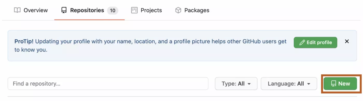
I. Create a meaningfully-named GitHub repository

In GitHub, click on Repositories and then click New:

Repositories.png

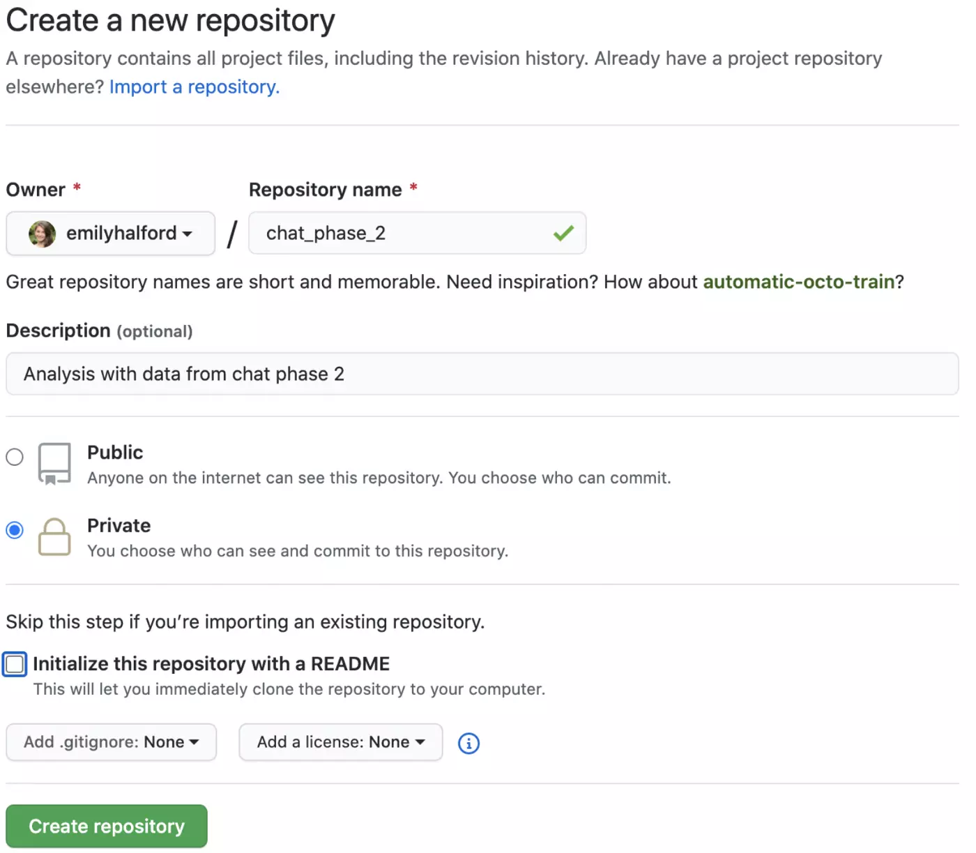
From there, you can give your repo a name and brief description. This repo contained data from the second phase of a study using online chat data, and has therefore been named “chat_phase_2.” I know that this name will allow me to find the repo if I come back to it several months later, and that my collaborators will be able to keep track of it as well.

Your repo can either be public (anyone can find your repo and its contents) or private (only you and designated collaborators can see it and its contents). There are many great uses for public repos (e.g. sharing packages you create, sharing cool projects you create) but if you are using data that contains confidential information and/or are conducting research that has not yet been published, you ALWAYS want to use a private repo. You can change these designations later, but should always be careful about what information you make public.

Typically, you will want to create a README file to guide yourself and anyone else who might access your repo through its contents. A good README outlines the contents of your repo, as well as providing a brief rationale for the work you’ve done.

New_Repository.png

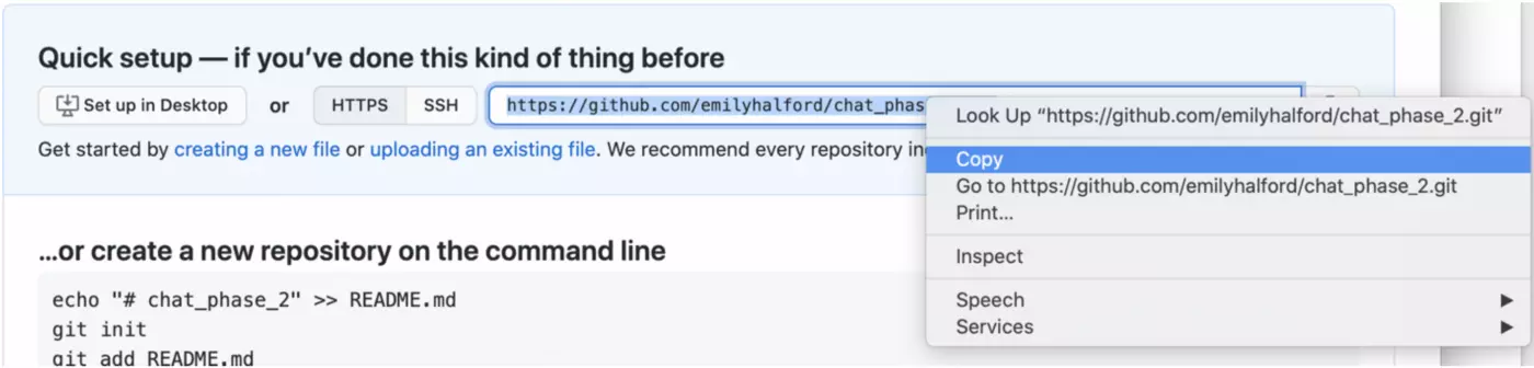
Click “create repository”, and then copy the link that will appear on the following page:

Click_create_repository.png

II. Create a new project in R and link it to this repo

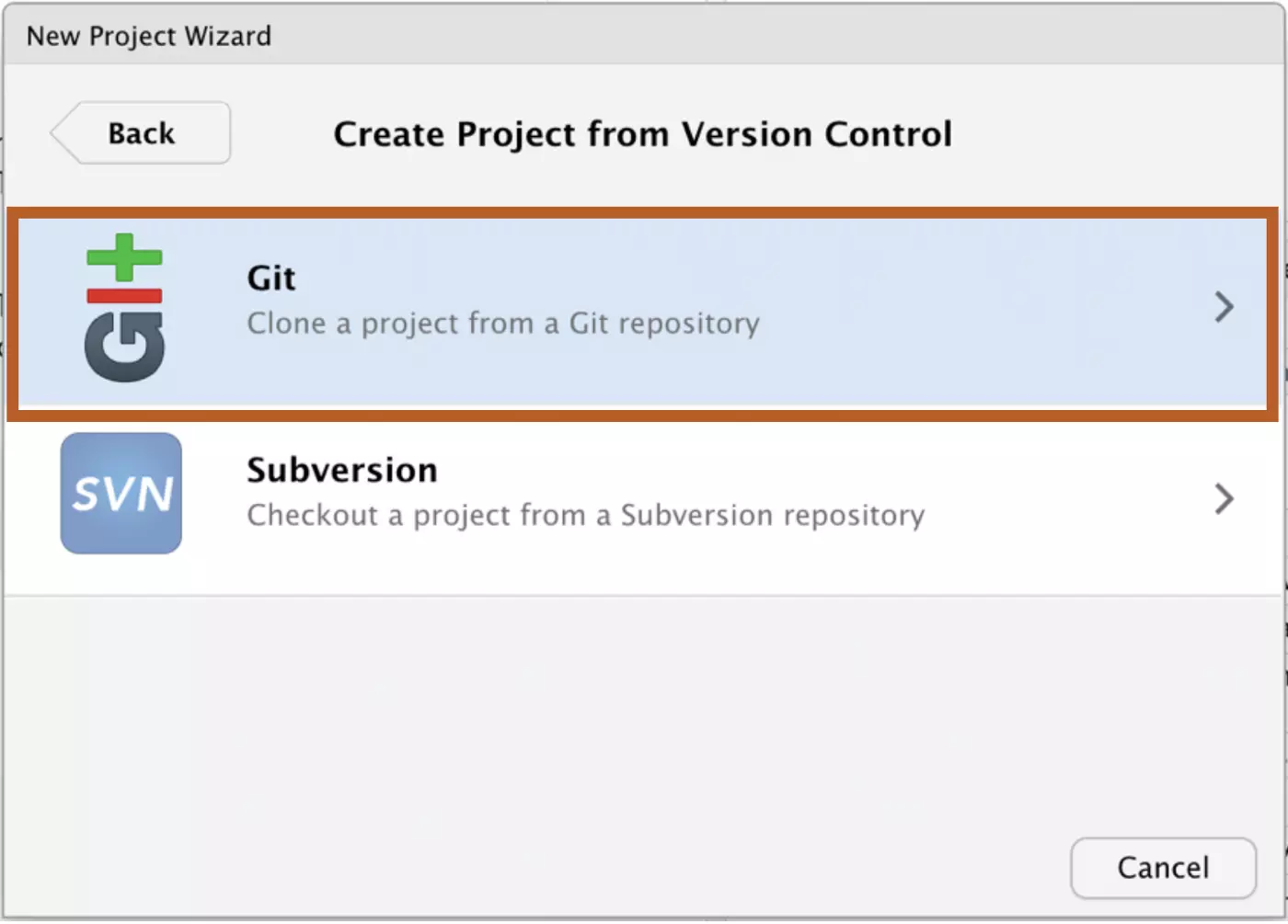
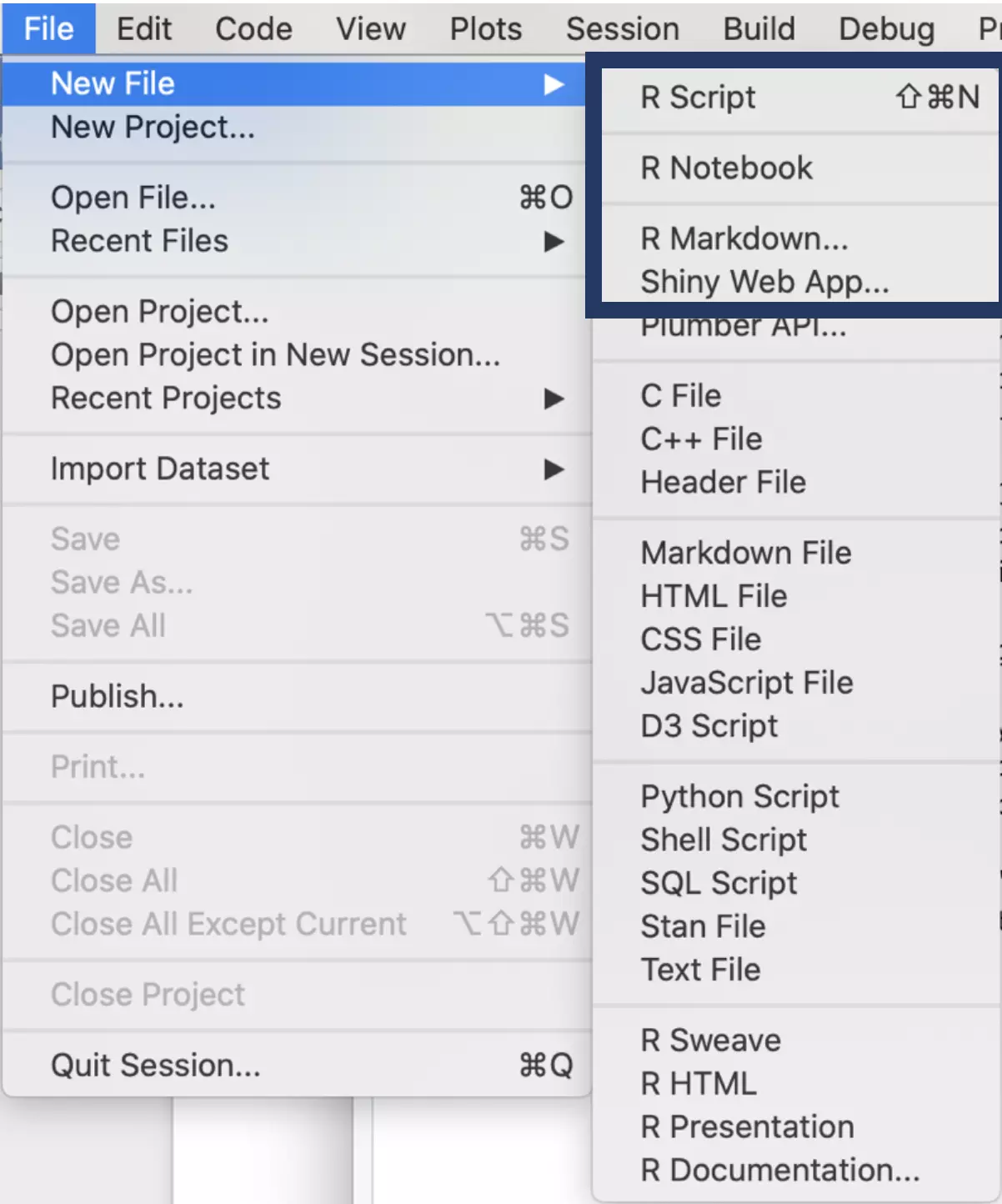
In R, click File → New Project

Next, select “Project with version control”:
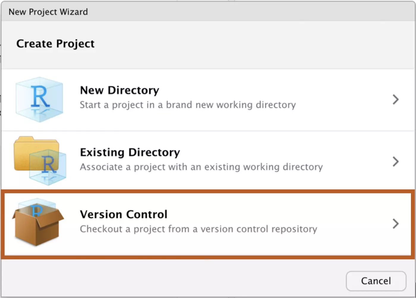
New Project Wizard

Select Git:

Select_Git.png

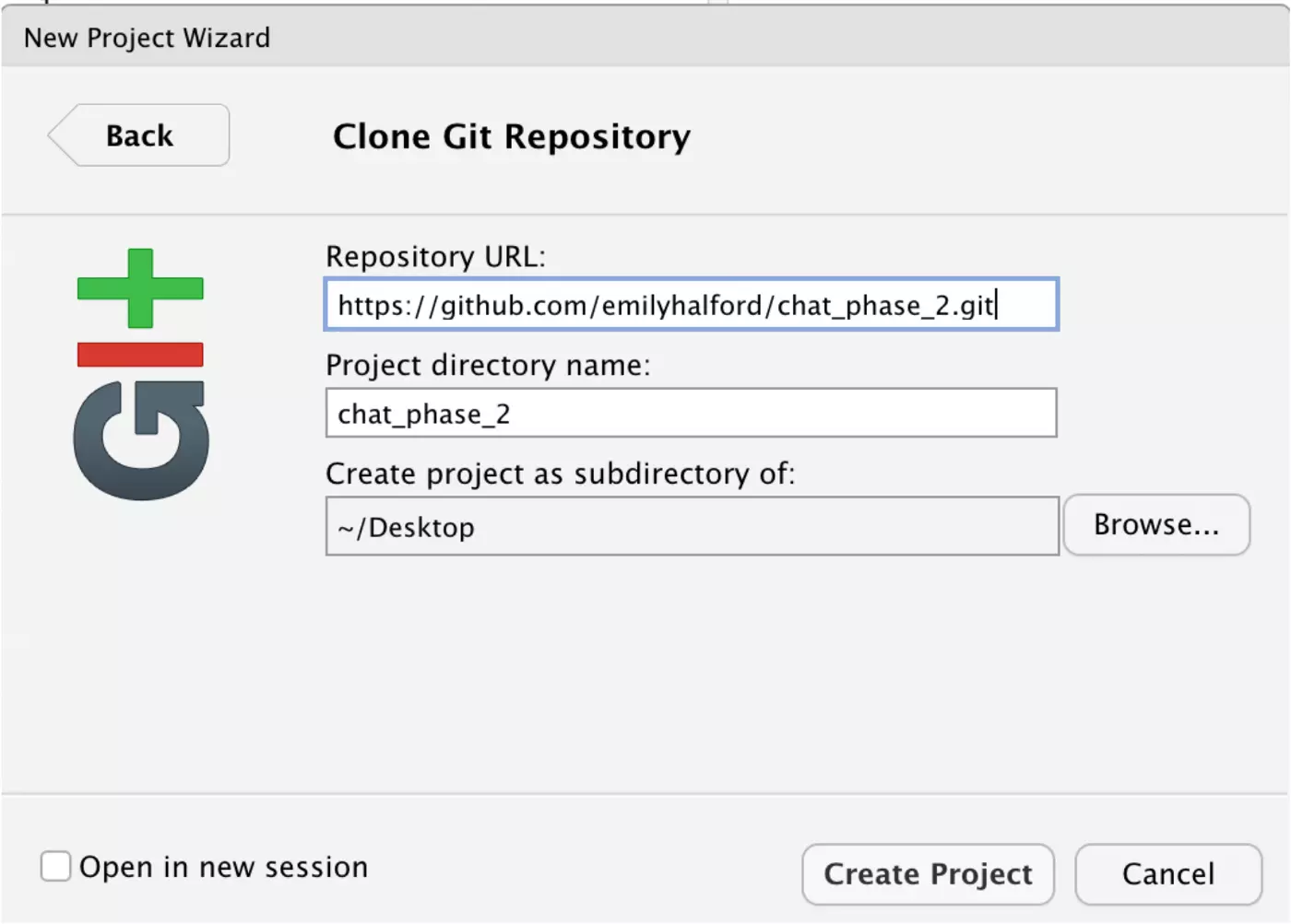
Finally, paste the URL that you copied from GitHub under Repository URL and click “Create Project”. I’ve created my project folder on my desktop, but you can browse to create your project anywhere on your computer.

Clone Git Repository

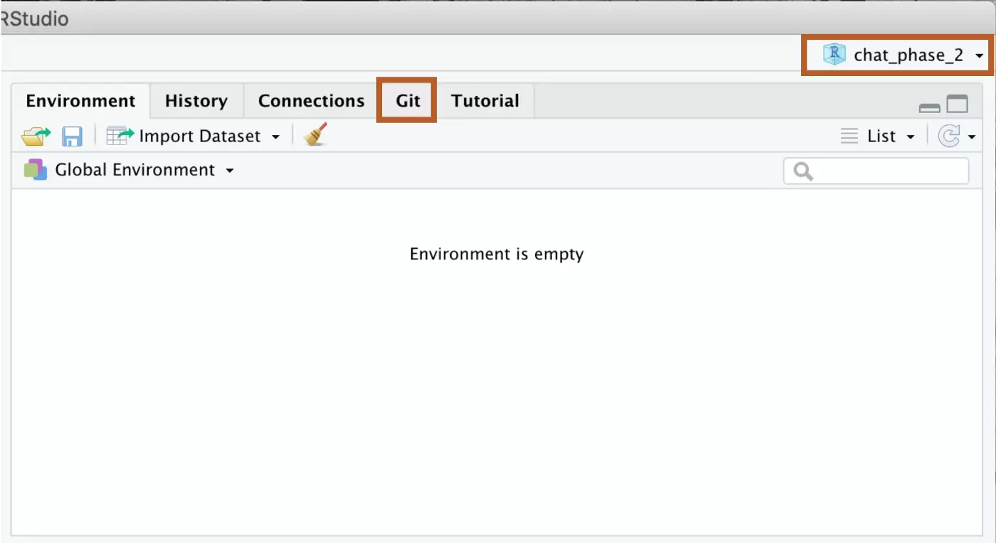
The project should open in R. You’ll know that it worked because your project will be indicated as the open project in the upper right corner of the screen, and you will now have a “Git” tab in the upper right panel.

RStudio.png

III. Store all related files in this project folder with meaningfully-named, consistent subfolders (such as a “data” folder that stores all of your data)

Now that you’ve created a local project and a GitHub repo, you’ll want to keep these clean and organized as you progress.

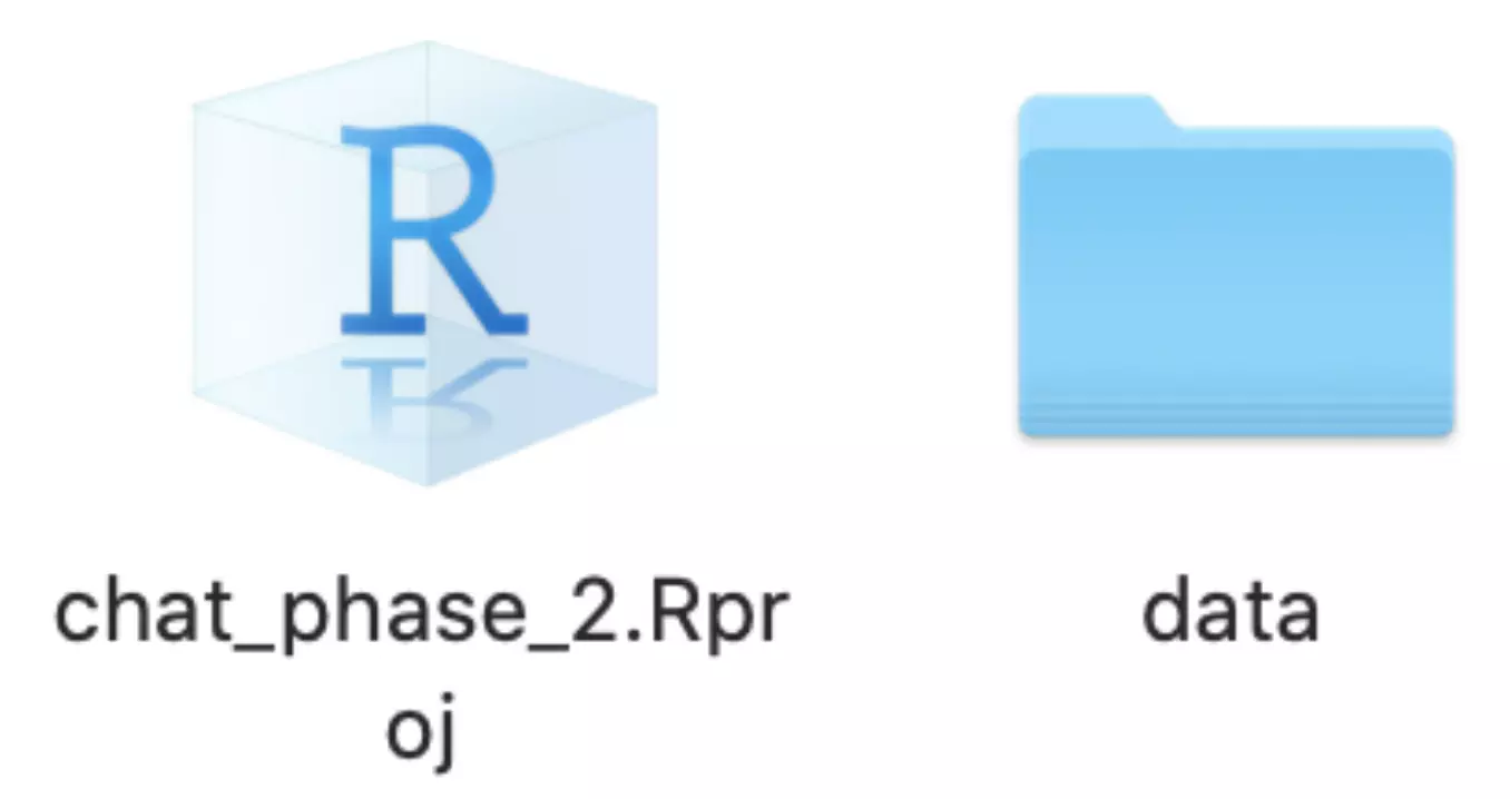
I added my data to the project in a data folder, so my current project folder looks like this:

Data_Project.png

As I progress, any additional data will be added to this “data” folder with consistent file names, I will create an “output” folder for any important graphs or other output that I create, and I will have several R Markdown files that are intentionally divided. For example, I may have one Markdown file where I clean data, one where I perform analyses, and one where I generate visualizations.

IV. Use the Git tab in R to consistently knit, commit, and push

GitHub only works for version control if you consistently push your work to their platform. In order to do this, click on the “Git” tab in RStudio. Any time you make changes to your local project, they’ll appear under this tab. First, click all of the changes that you’ve made since you last updated the repo. Next, click the “Commit” button.

Commit.png

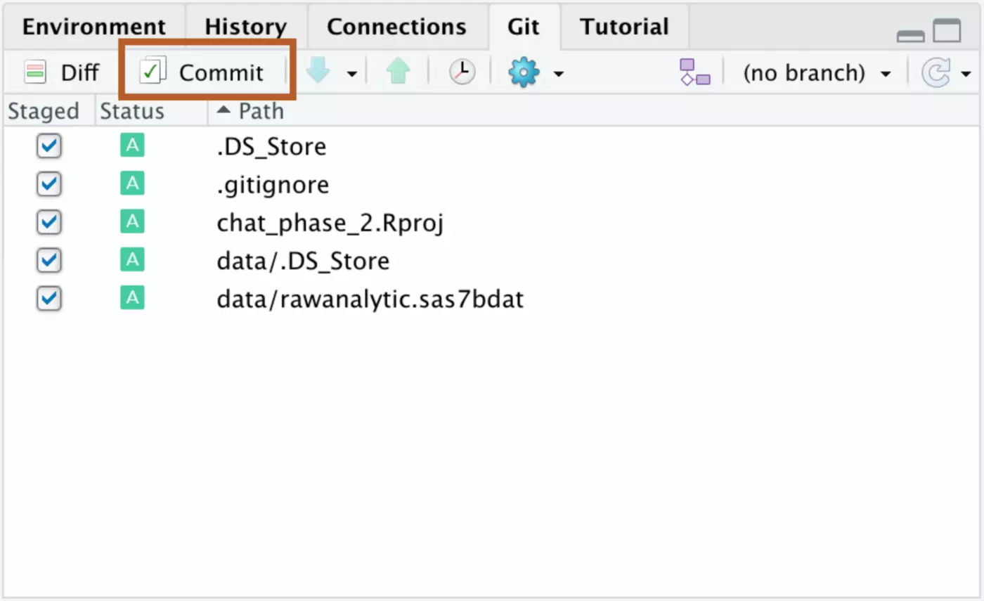
You will want to enter a commit message that describes the changes you are making. This makes it far easier for somebody else to navigate your repo, and will also make it easier to locate a previous version of your code if you need to access it later.

Once you’ve entered a commit message, select “Commit” in the bottom right corner. If that runs without error, the “Push” button will be accessible. Click “Push” to send your updates to GitHub.

Review_Changes.png

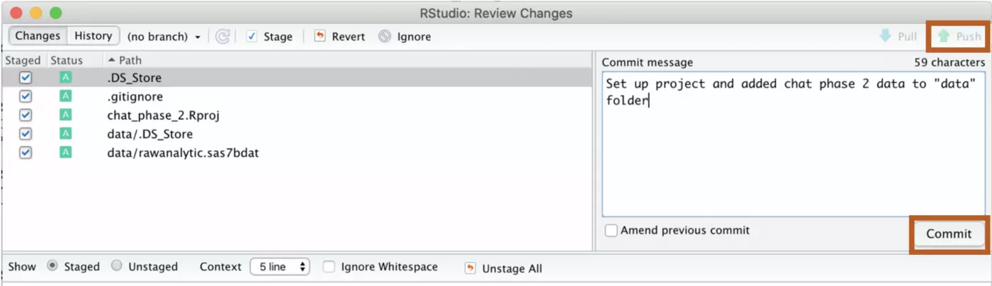
Now all of your changes are backed up on GitHub! You will want to do this consistently as you work. I recommend checking out your GitHub account the first time you do this to see how your work is stored there. If you are accessing somebody else’s repo, or if somebody else has made changes to yours, you can use “Pull” to pull the latest version of the repo to your computer.


5. Loading Packages

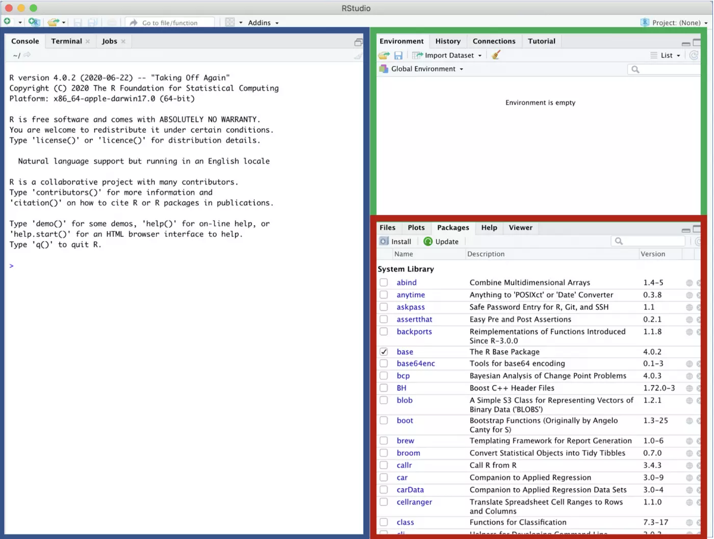
Now that everything is set up, you can start working in R!

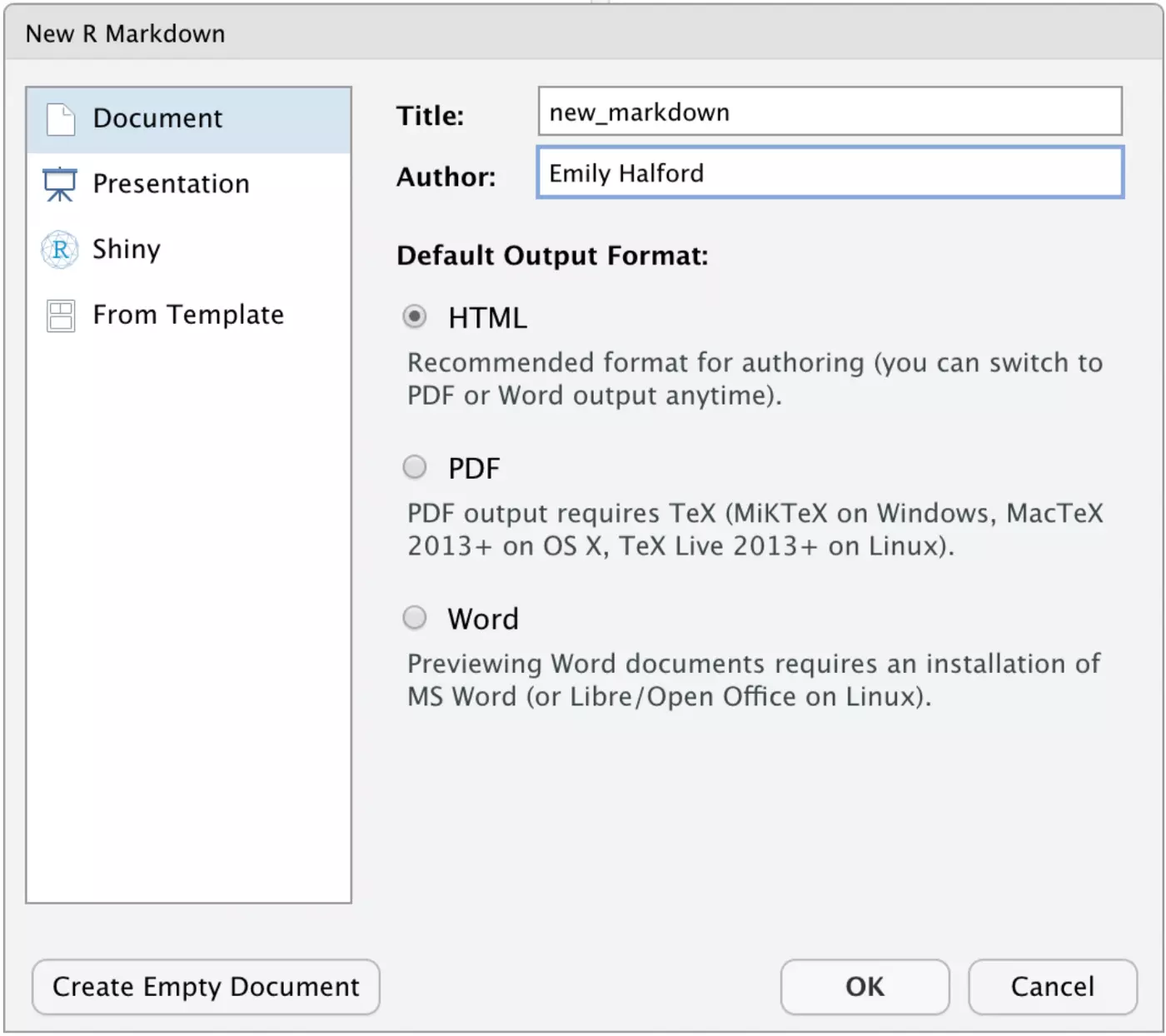
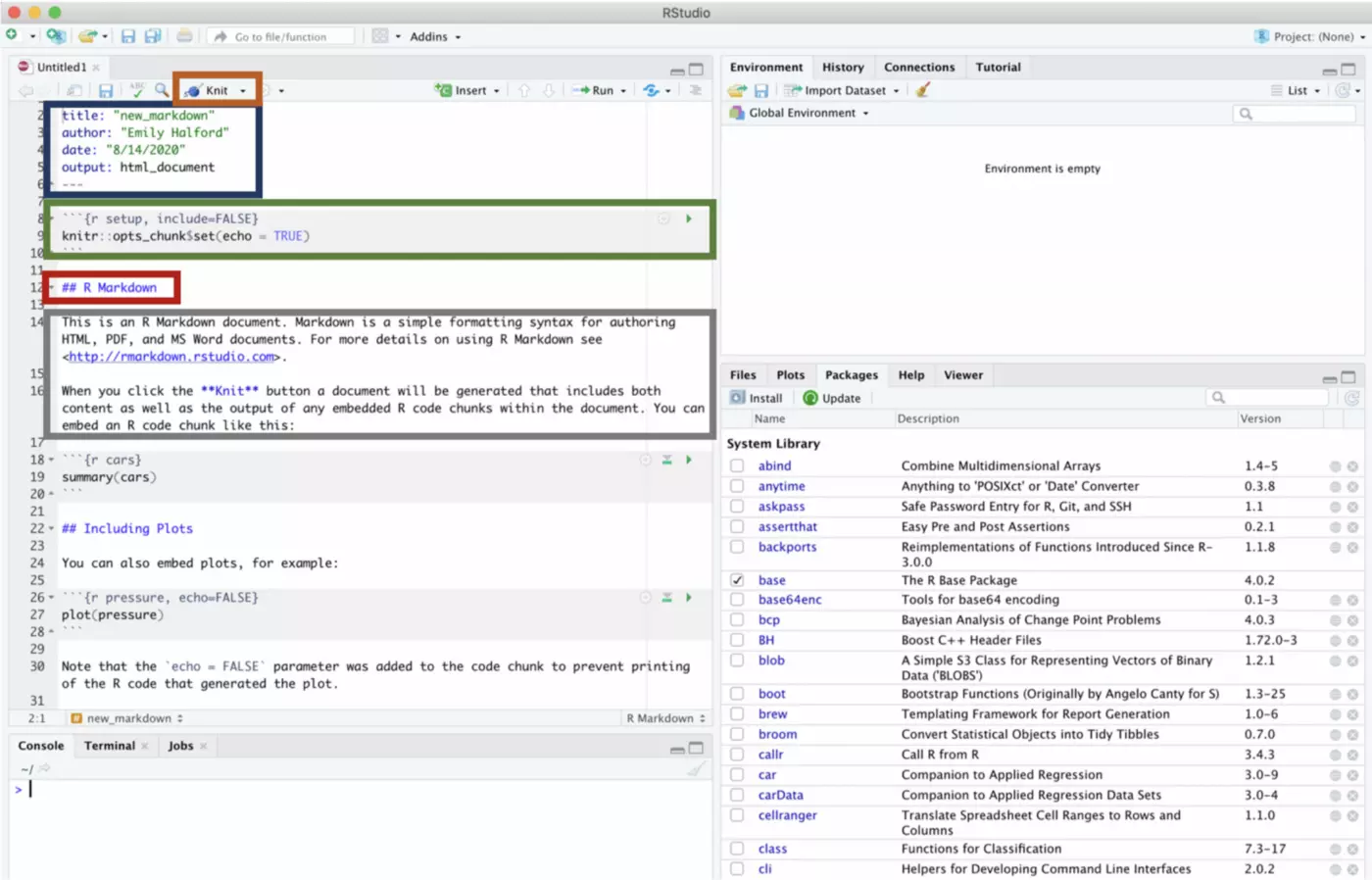
First, open up a new R Markdown file. If you click File → New File → R Markdown while your project is open (again, you can tell that your project is open if its name is in the top right of your window), the R Markdown file will be created in your project automatically.

R automatically comes with “base R” functions. However, R is open-source (meaning that anyone can contribute packages), and there are a lot of amazing packages out there that you will need to use R efficiently. You will have to install these packages one time, and then load them every time that you want to use them. The code for doing so is provided below (note the double quotation marks to install a package and single quotes to load it). I like to install packages in the console, as I only have to do this once and therefore have no reason to save the line of code which installs the package. You will see confirmation in the console that the package has installed and loaded correctly.

install.packages.png

Note: Tidyverse is actually a collection of packages rather than a single package. I highly, HIGHLY recommend familiarizing yourself with tidyverse and the packages included within it. They are widely used and are popular because they will make your life infinitely easier — I automatically load it every time I create a new Markdown file. You can find more information about tidyverse and its component packages here: https://www.tidyverse.org/
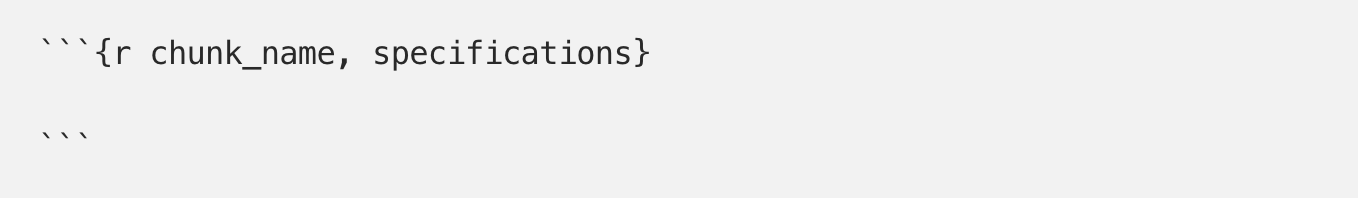
6. Other Notes

R is case-sensitive, unlike SAS and some other languages. This case-sensitivity is one of the reasons it’s so important to use consistent file- and variable-naming structures — you’ll be less likely to have annoying errors in your code and anyone else looking at your code will be more able to follow it. Personally, I use snake case (everything_is_lowercase_with_underscores) exclusively.

There are also established guidelines for how you should format your code. You should strive for code that not only runs, but is also tidy! One useful style guide from Hadley Wickham can be found here: http://adv-r.had.co.nz/Style.html

7. Up and Running!

You should now be able to open a new R Markdown file as part of an intentional workflow and to install and load packages within that file. These skills set you up to make even better use of the fantastic tutorials out there than can walk you through importing, cleaning, analyzing, and visualizing your data in R.

Share this article

Leave your comments

Post comment as a guest

0
terms and condition.
  • Michael Holms

    Outstanding article !!!!

  • Amit Jain

    Excellent guide! I found this article to be way more beneficial than anything else I've read on the topic.

  • Steve Hackney

    As a beginner I am struggling to figure out R... This tutorial is simply amazing....

  • Amit Jain

    In reply to: Steve Hackney

    I bookmarked this guide ! You should do the same !

  • Sam Dickson

    Clear STRUCTURE & Well PRESENTED. Thx

  • Cassy Bank

    So much value in one single article! Warming up for my job interview in data science!

  • Cassy Bank

    Great tutorial!

  • Andy Morrison

    Very concise, organized, and clearly explained. I wish all guides were this well done.

  • Thomas K

    Ideal for beginners and even for those that are experienced!

  • Yang Zhang

    What an amazing tutorial!!Thank you so much Emily. I can't thank you enough.

  • Min Soo Kim

    Excellent tutorial

Share this article

Emily Halford

Data Science & Mental Health Expert

Emily is a data analyst working in psychiatric epidemiology in New York City. She is a suicide-prevention professional who is enthusiastic about taking a data-driven approach to the mental health field. Emily holds a Master of Public Health from Columbia University.

   
Save
Cookies user prefences
We use cookies to ensure you to get the best experience on our website. If you decline the use of cookies, this website may not function as expected.
Accept all
Decline all
Read more
Analytics
Tools used to analyze the data to measure the effectiveness of a website and to understand how it works.
Google Analytics
Accept
Decline