The Janitor Package
The janitor package is available on CRAN and was created by Sam Firke, Bill Denney, Chris Haid, RyanKnight, Malte Grosser, and Jonathan Zadra. While arguably best known for its extraordinarily useful clean_names() function (which I will be covering later on in this article), the janitor package has a wide range of functions that facilitate data cleaning and exploration. The package is designed to be compatible with the tidyverse, and can therefore be seamlessly integrated into most data prep workflows. Useful overviews of janitor package functions that I have consulted can be found here and here. Additionally, all data and code referenced below can be accessed in this GitHub repo.
GNIS Data
The data that we will be using in this tutorial comes from the Geographic Names Information System (GNIS), a database created by the U.S. Board on Geographic Names. This dataset was featured in Jeremy Singer-Vine’s Data is Plural newsletter, and is essentially a searchable catalogue of domestic place names.
In order to download the data, we will first need to navigate to the Query Form:
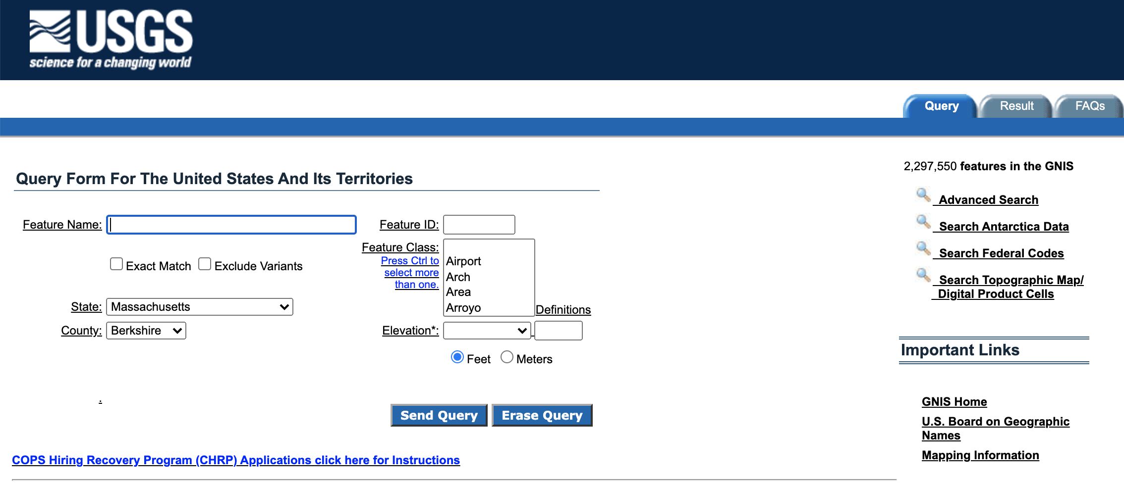
I chose to utilize data representing place names in Berkshire County, Massachusetts, a region that includes my hometown. In order to create this search, select “Massachusetts” from the state drop-down menu and “Berkshire” from the county drop-down menu. Then, click the “Send Query” button:
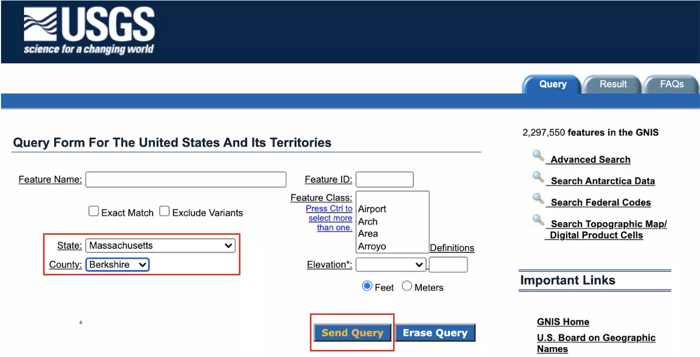
The query results will appear as shown below. Beneath the results table, click ‘Save as pipe “|” delimited file’ to save the data locally:
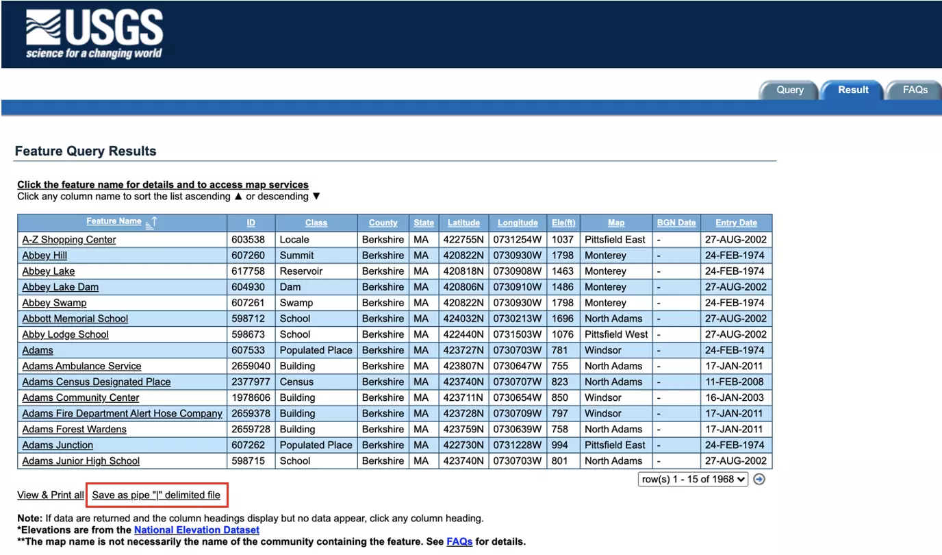
The data should begin to download automatically, and will appear in a .csv file with features delimited by “|”:
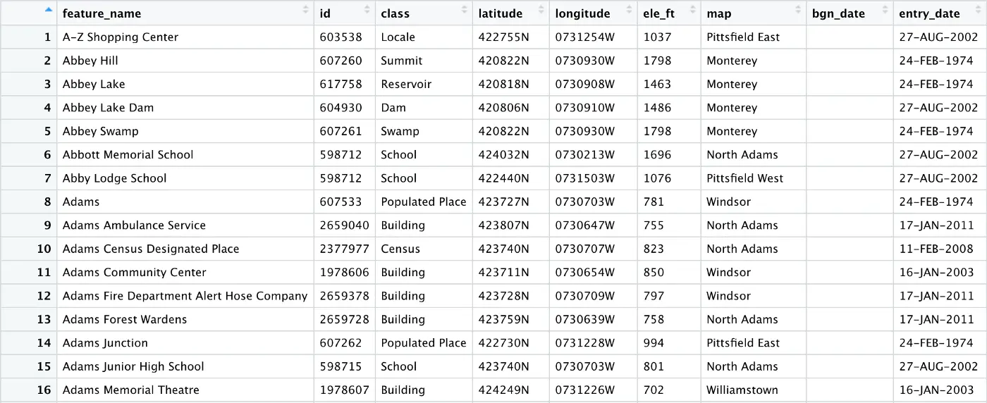
Save this csv file into a “data” folder in a new R project. Let’s bring the data into R, separate these columns out, and perform a bit of modification to facilitate our janitor package exploration. First, load the tidyverse and janitor packages in a new R Markdown file. Use the read.csv() function to load in the data as “place_names”:
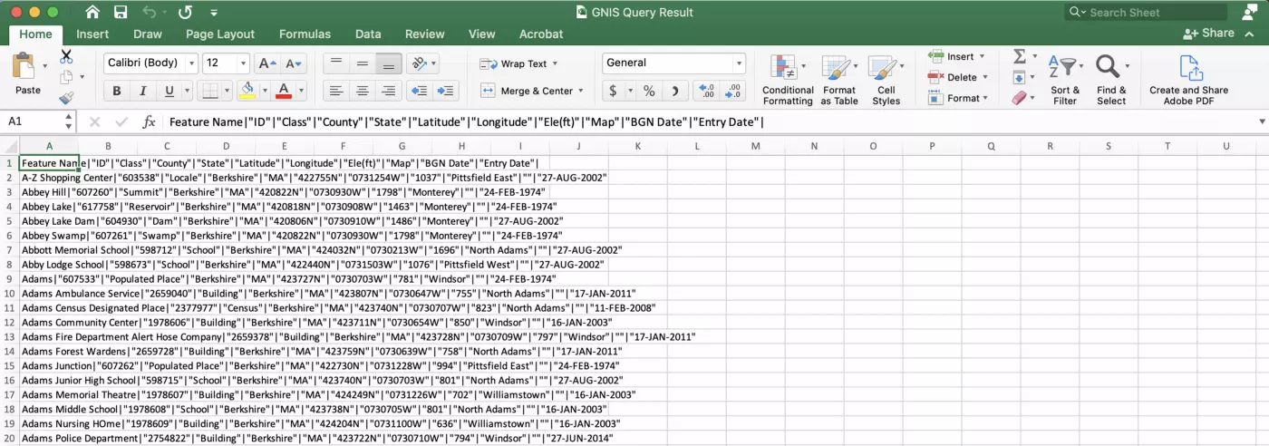
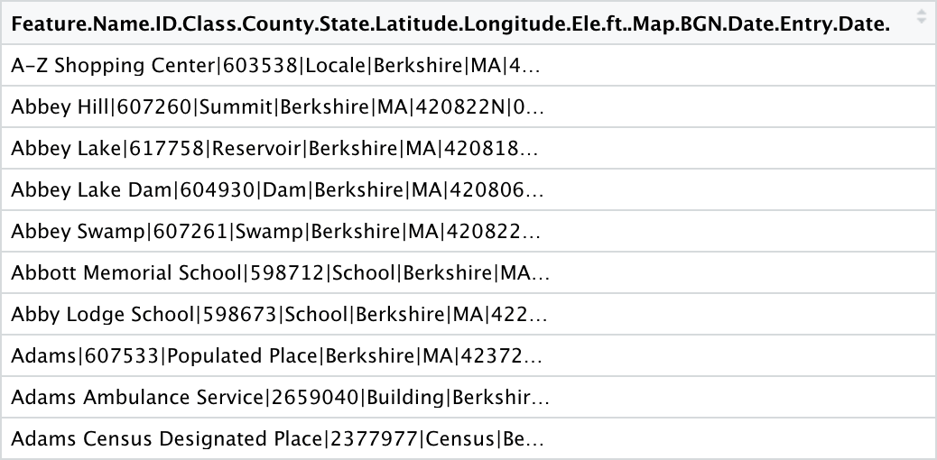
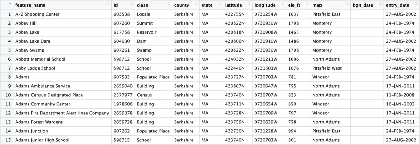
The data should look pretty much the same as it did in Excel, with one massive column containing all of our data:
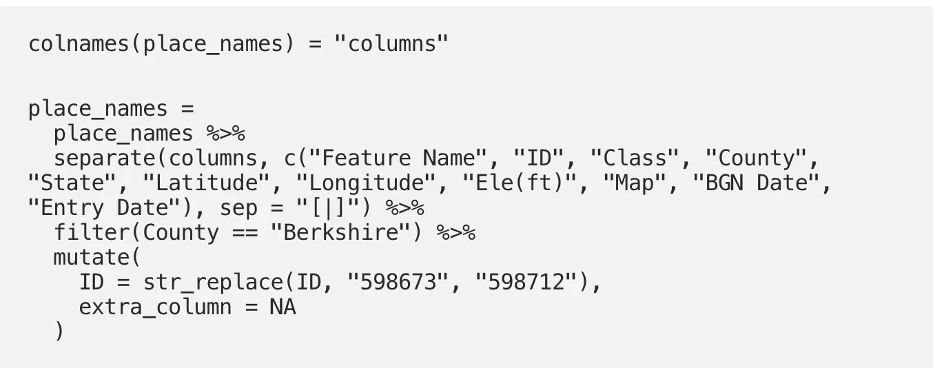
Let’s work with this a bit. First, we assign the name “columns” to this single column to avoid having to include something as messy and long as the default column name in our code. Next, we use the separate() function to separate this one column into all of its component parts. We then filter the data down to Berkshire County, as upon further inspection of the data it becomes clear that a few entries from outside this county were included in our Berkshire County query. We then dirty the data a bit in a mutate() step so as to tidy it later. str_replace() is used to replace the ID “598673” with “598712,” an ID number that already exists in the dataset, in order to create a duplicate ID. Finally, an extra column called “extra_column” is created with NAs in every row:
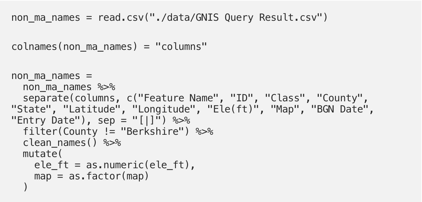
Before moving on, let’s quickly create a second data set called “non_ma_names” containing those entries that were not actually from Berkshire County. Yet again we read in the “GNIS Query Result.csv” file and separate out the column names. We then apply the clean_names() function from the janitor package, which we will cover in depth in the following section. Finally, we use as.numeric() and as.factor() in a mutate step to transform our ele_ft variable to an numeric variable and our map variable to a factor:
Now let’s see what janitor can do!
Using janitor
row_to_names()
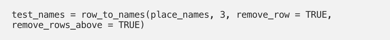
You’ve probably received plenty of data files, likely in .xlsx form, that have several rows at the top of the spreadsheet before the actual data begins. These rows may be blank, or filled with information and corporate logos. When you load such data into R, content from these leading rows may automatically become your column headers and first rows. The row_to_names() function in the janitor package allows you to indicate which row in your data frame contains the actual column names and to delete everything else that precedes that row. Conveniently for us, the GNIS data already had column names in the correct place. Let’s try this out anyway, though, pretending that the column names were actually in the third row.
We use the row_to_names() function to create a new data frame called “test_names”. The row_to_names() function takes the following arguments: the data source, the row number that column names should come from, whether that row should be deleted from the data, and whether the rows above should be deleted from the data:
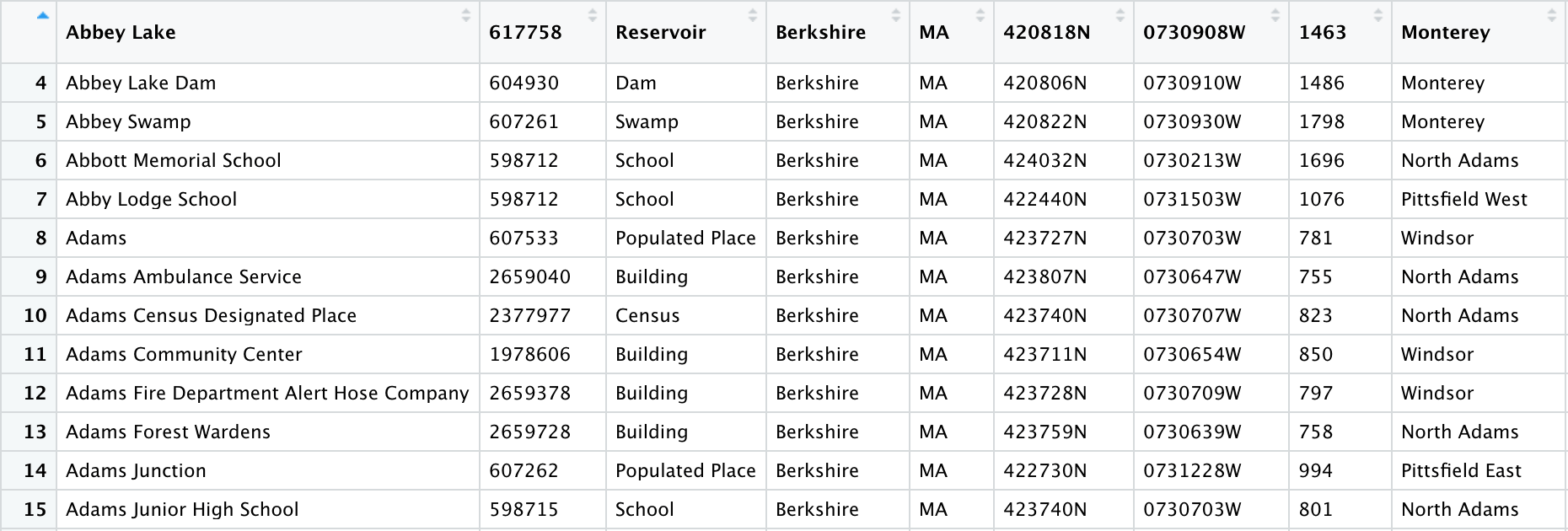
We can see that the information from row 3 now makes up our column names. That row and those above it were removed from the data frame, and we can see that the data now begins on row 4:
While this function isn’t necessary to clean the GNIS data, it certainly comes in handy with other data sets!
clean_names()
This function is one that I use almost every time I load a new dataset into R. If you’re not already using this function, I highly recommend incorporating it into your workflow. It’s the most popular function from this package for a reason — it’s extremely useful!
The tidyverse style guide recommends snake case (words separated by underscores like_this) for object and column names. Let’s look back at our column names for a minute. There are all sorts of capital letters and spaces (e.g. “Feature Name,” “BGN Date”) as well as symbols (“Ele(ft)”). The clean_names() function will convert all of these to snake case for us.
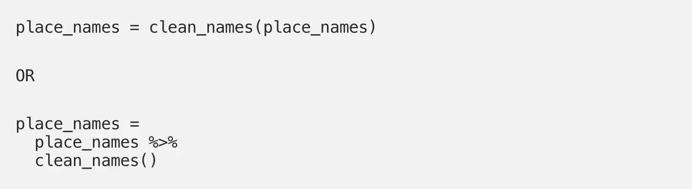
Using clean_names() is as easy as follows:
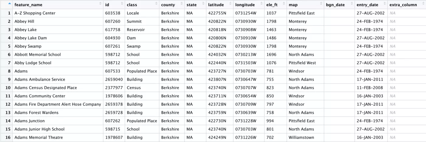
As you can see below, this one function handled every kind of messy column name that was present in our data set. Everything now looks neat and tidy:
remove_empty()
The remove_empty() function, as its name suggests, deletes columns that are empty. We created an empty column in our “place_names” data frame while prepping our data, so we know that at least one column should be impacted by this function. Let’s try it out:
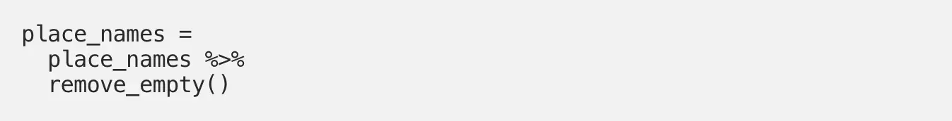
As you can see, the empty_column has been dropped from our data frame, leaving only columns that contain data:
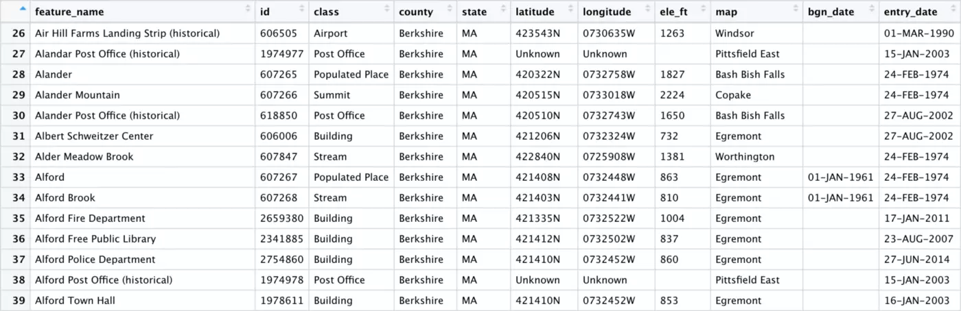
The bgn_date column looks empty, but the fact that it was not dropped by remove_empty() tells us that there must be data in at least one row. If we scroll down, we see that this is in fact the case:
remove_constant()
The remove_constant() function deletes columns with the same value in all rows. Our dataset currently has two of these — since we filtered the data down to Berkshire County, and all of Berkshire County is within Massachusetts, county = “Berkshire” and state = “MA” for all rows. These rows aren’t particularly useful to keep in the dataset since they provide no row-specific information. We could simply use select() to drop these columns, but the benefit of remove_constant() is that this function double-checks the assumption we’re making that all entries are the same. In fact, using remove_constant() was how I first discovered that 38 out of 1968 entries in the raw data weren’t actually from Berkshire Country!
Like remove_empty(), all the information that the remove_constant() function needs is the dataset it should act on:
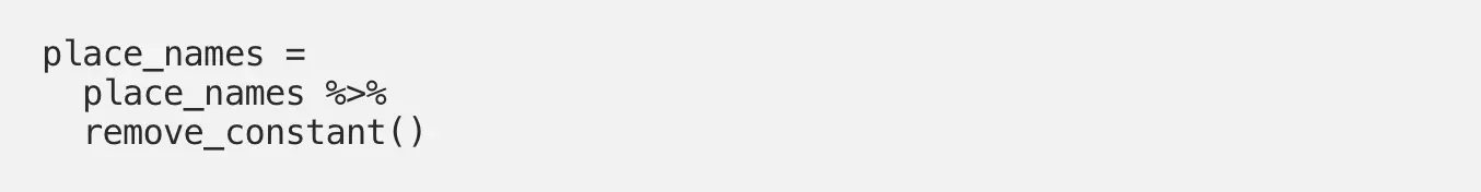
As you can see below, the county and state columns have been dropped:
compare_df_cols()
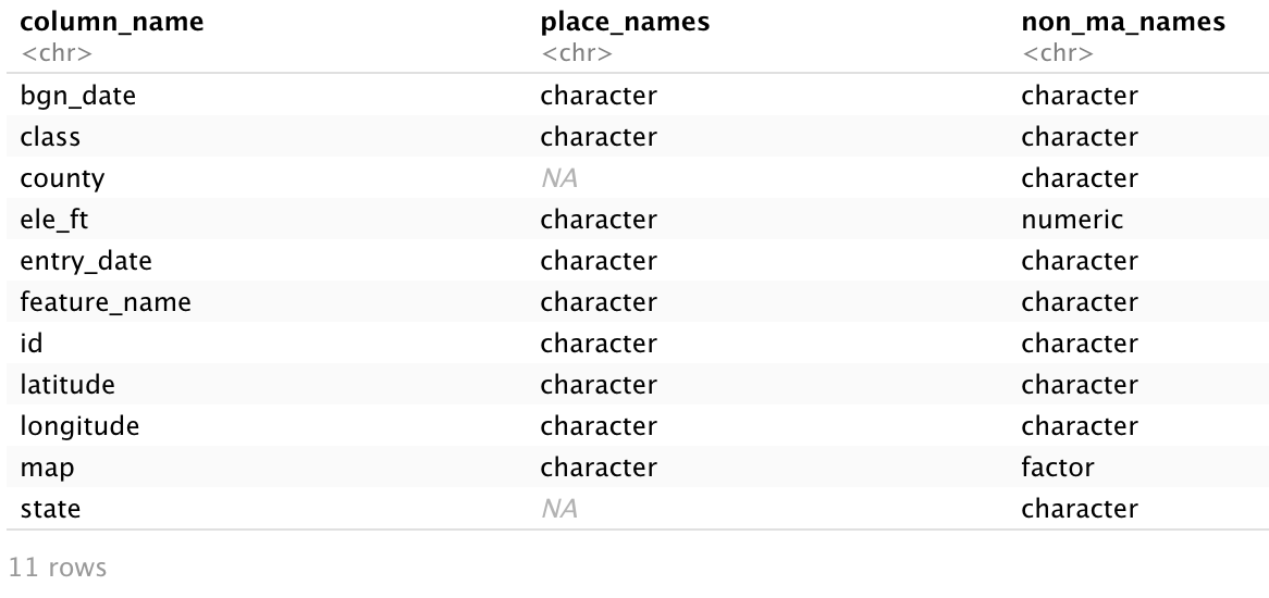
Ever try using rbind() to stack two data frames together and run into an unexpected error? The compare_df_cols() function directly compares the columns in the two data frames and is incredibly useful for troubleshooting this problem. Let’s try it out by comparing our “place_names” data frame to the data frame that we created containing entries outside of Berkshire County, “non_ma_names”:

The output is a convenient table comparing the two data frames. We see “NA” for county and state in place_names and “character” for these variables in non_ma_names. This is because we deleted these columns with remove_constant() from place_names, but never did anything to the default character variables in non_ma_names. We also see ele_ft as numeric and map as a factor variable in non_ma_names, which we specifically designated during data prep. If we were trying to merge these data frames back together, it would be useful to know which columns are missing as well as which columns have inconsistent types across data frames. In data frames with many columns, compare_df_cols() can significantly reduce the time spent making these comparisons.
get_dupes()
I’ve frequently worked on projects with unique patient IDs that you do not expect to see duplicated in your dataset. There are plenty of other instances when you might want to make sure that some ID variable has entirely unique values, including our GNIS data. As you’ll recall, we created a duplicate ID when prepping our data. Let’s see how get_dupes() detects this. The function just needs the name of our data frame and the name of the column acting as an identifier:

As shown below, the data frame is filtered down to those rows with duplicate values in the ID column, making it easy to investigate any problems:

tabyl()
The tabyl() function is a tidyverse-compatible replacement for the table() function. It is also compatible with the knitr package, and is quite useful for data exploration.
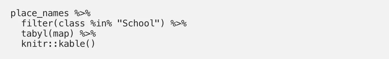
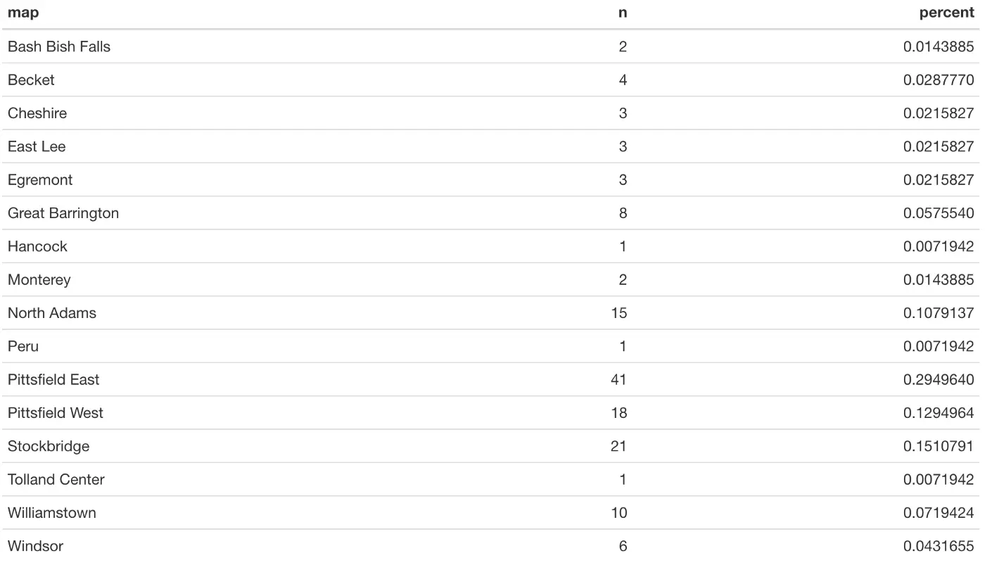
Let’s try it out first with a single variable. Say we’re interested in how many schools are in each of the towns in Berkshire County. We first filter our class variable to “School,” then use the tabyl() function with our map (location) variable. Finally, we pipe that into knitr::kable() to format the output in a nice table:
Running this very basic code chunk produces the following output table:
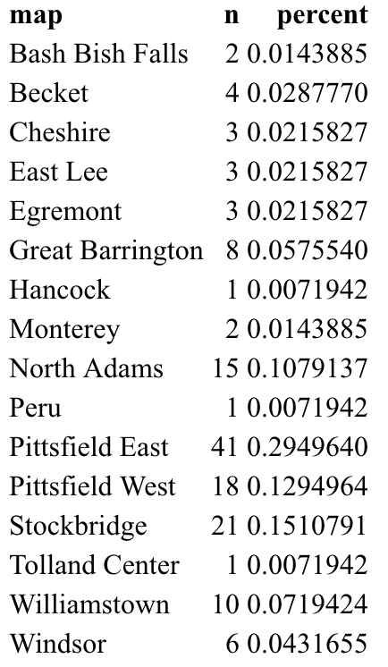
When we knit our Rmd file, the kable() function will have formatted the table nicely, as shown below. We conveniently get a count of schools in each town, as well as the percentage of all schools that are in that town. It’s easy to make observations about these data, such as that 29.5% of all schools are in Pittsfield East, which has 41 schools. Or that 3 towns are so small that they only have 1 school:
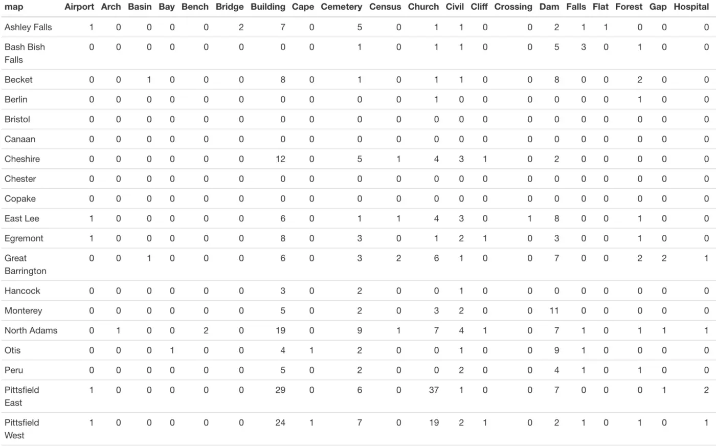
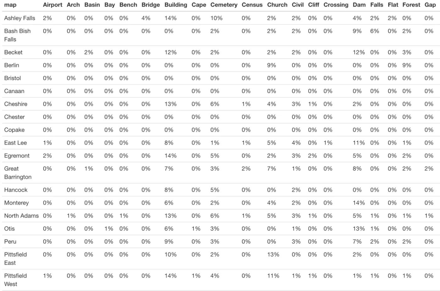
Now let’s try the cross-tabulation of two variables. Let’s see how many landmarks of each type are present in each town:
A portion of our table (once knitted) is shown below. For each town, we can clearly see how many of each landmark type are in the database:
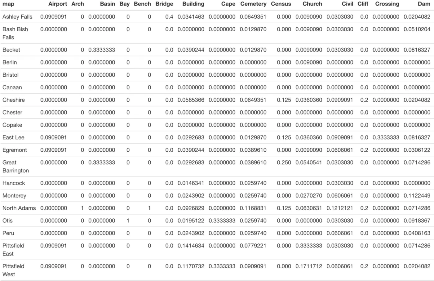
While simple counts like this can be quite useful, maybe we care more about column percentages. In other words, what percentage of entries for each landmark type are in each town? This is easy to investigate with tabyl() via the “adorn_percentages()” function:
Now we see these column percentages instead of counts, but the table is rather difficult to read:
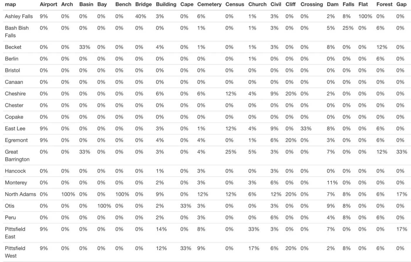
We can clean this up a bit with the adorn_pct_formatting() function, which allows the user to specify the number of decimal places to include in the output. Precision isn’t particularly important for this exploratory table, so let’s use 0 decimal places to make this table easier to read:
Much better! Now it is much easier to read the table and understand our column percentages:
It is just as easy to use adorn_percentages() to instead look at row percentages (in our case, the percentage of entries from each town belonging to each landmark type):
Other Functions
In this article I have described the functions from the janitor package that I find useful in my day-to-day work. However, this is not an exhaustive list of janitor functions and I recommend consulting the documentation for further information on this package.
That being said, there are a few other functions that are worth at least noting here:
- excel_numeric_to_date(): This function is designed to handle many of Excel’s date formats and to convert these numeric variables to date variables. It seems like a big time saver for those who frequently work with data in Excel. As an infrequent Excel user, I instead rely heavily on the lubridate package for working with date variables.
- round_to_fraction(): This function allows you to round decimal numbers to a precise fractional denominator. Want all of your values rounded to the nearest quarter, or are you using decimals to represent minutes in an hour? It’s likely that the round_to_fraction() function can help you.
- top_levels(): This function generates a frequency table which collapses a categorical variable into high, middle, and low levels. Common use cases include simplifying Likert-type scales.
Conclusion
It’s common knowledge at this point that most data analysts and data scientists devote a majority of their time to data cleaning and exploration, and I therefore always find it exciting to discover new packages and functions that make these processes a little more efficient.
Whether or not you have previously used the janitor package, I hope that this article has introduced you to some functions that will prove to be useful additions to your data science toolkit.


Leave your comments
Post comment as a guest